One of the things that I find most remarkable about science is how often disparate phenomena are connected in deep ways. The first two items in the title of this post are examples of a phase change. When the attractive forces between molecules, or the alignment of magnets, exceed the randomizing effects of temperature the system falls into a large scale order to form a solid or a ferromagnet.
There is also a strong mathematical connection to the epidemiology of a pandemic. The ability of an illness to spread is, in the abstract at least, just like the ability of magnets to align together or water molecules to freeze into a block of ice.
The study of phase changes is mathematically complex. One of the first, and simplest, techniques used to study this topic is called the Ising Model. It was constructed by Wilhelm Lenz in an attempt to model the formation of magnetic domains and assigned to his student, Ernst Ising. The model imagines a set of magnets that interact only with their nearest neighbor. Ising solved the simplest case, a one dimensional line, in his 1924 Ph.D. thesis, where he showed that there was no phase transition. He incorrectly concluded that the model was not able to produce a phase transition in any number of dimensions. The more complex two dimensional model was shown to have a phase transition by Rudolf Peierls in 1936 and solved by Lars Osanger in 1944. (The link in the previous sentence should not be followed by the mathematically timid) This shows a phase transition.
In its simplest form neighboring elements are given a probability of being aligned. Think of it as tiny magnets that have a tendency to face the same way but the random vibrations due to not being at absolute zero make this less than certain.
The correlation of the magnets works out to be given by a mathematical function that deserves far more familiarity than it has; Hyperbolic Tangent (tanh). It looks like this:
The smooth transition from one state to the other doesn't seem like a good representation of a phase transition. But it is. The scale of the x axis changes with the number of elements in the simulation. For a large number of particles it looks like this:
One of the most surprising things, at least to me, is that freezing, or ferromagnetism, only happens if there are a large number particles involved. If the number of particles is small instead of there being a sudden transformation from one state to another at a well defined temperature there is a temperature range where the characteristics smoothly change from one state to the other. This behavior is captured very well by the Ising model.
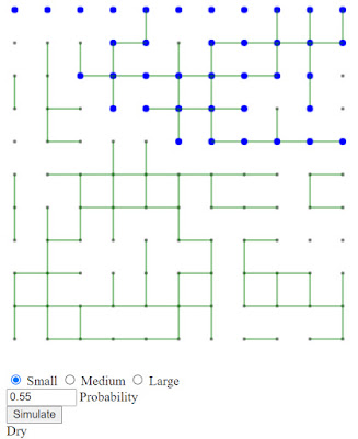
I've made an interactive webpage that shows a similar, but easier to compute system. Imagine a rectangular grid of points that can be connected by a pipe to the points on either side as well as above or below. Think of the top row as a source of water that can flow down, if the connections are there. The question is: Does the water make it to the bottom? Let's look at some examples to make it clear.
In this example there is a 10x10 grid with a 55% probability that any possible connection exists. In this case we see at the bottom of the image the word "Wet" indicating that (at least part of) the bottom row is "Wet". If we press "Simulate" sometimes the results are like the one above, other times like this:
If we run this many times with varying probability and note the fraction of the times the bottom is "Wet" at different probabilities. Here are some results for "small" grid with the probability setting ranging from 0.3-0.7:
The line is a tanh function adjusted to fit. It is
very good fit to the points especially since I just eye-balled the adjustments for the tanh function and the data points still have some random noise since I only let the simulations run for a few thousand trials. As we vary the probability of a connection being present from 0.3 to 0.7 the fraction of "wet" final states changes smoothly from 0 to 1.
If we select "Medium" or "Large" the simulation uses 100 x 100 or 100 x 1000 points. As predicted by the Ising model the transition gets sharper and sharper.
Medium Large
This is instructive when thinking about epidemiology because it highlights a very unintuitive fact. When the percentage of people needed for disease spread to stop, often called "herd immunity" is considered this is not a gradual change. It is very much like the ability of water in the model above to get to the bottom. With a large enough group of people there is a sharp difference between a population that is protected from disease spread and one that is not. If herd immunity requires say, 65% of the population to vaccinated, it isn't true that 60% is pretty close. The population is either herd immune or it isn't.


